#Tag · bonfire.cafe

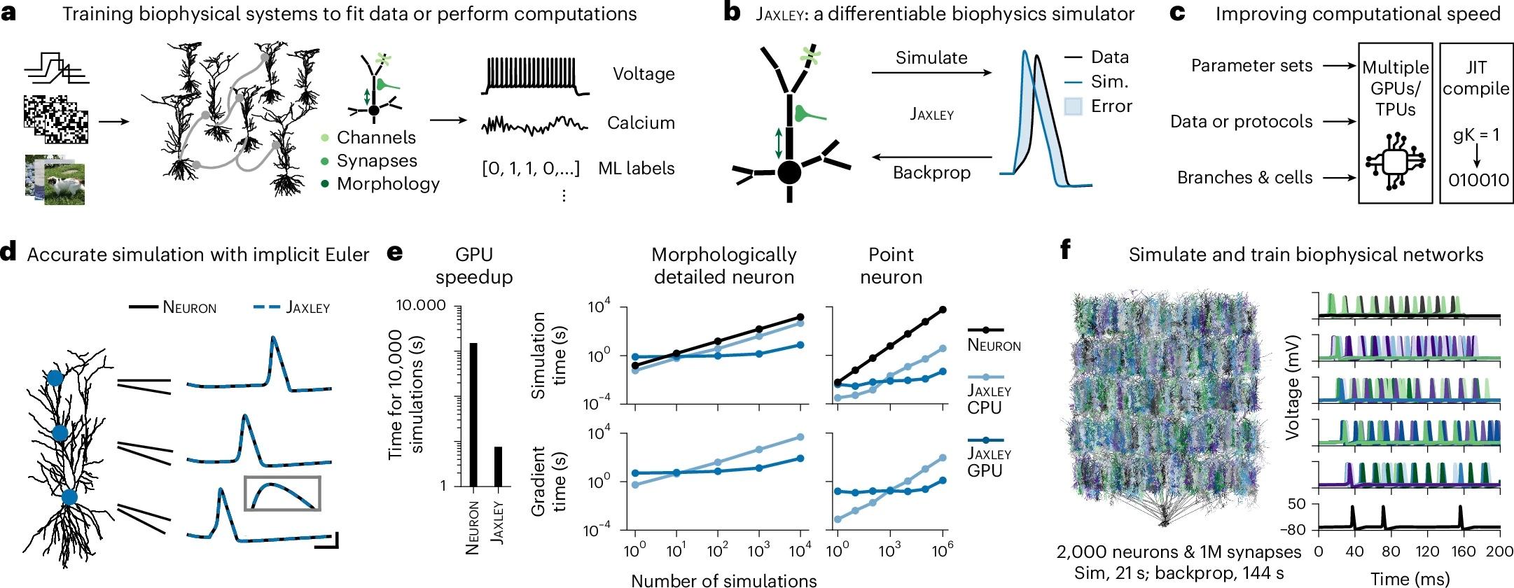
🧠 New paper by Deistler et al: #JAXLEY: differentiable #simulation for large-scale training of detailed #biophysical #models of #NeuralDynamics.

They present a #differentiable #GPU accelerated #simulator that trains #morphologically detailed biophysical #neuron models with #GradientDescent. JAXLEY fits intracellular #voltage and #calcium data, scales to 1000s of compartments, trains biophys. #RNNs on #WorkingMemory tasks & even solves #MNIST.

🌍 https://doi.org/10.1038/s41592-025-02895-w

#Neuroscience #CompNeuro

Jaxley: differentiable simulation enables large-scale training of detailed biophysical models of neural dynamics

Fig. 1: Differentiable simulation enables training biophysical neuron models.

Fabrizio Musacchio

@pixeltracker@sigmoid.social · 2 days ago

🧠 New paper by Deistler et al: #JAXLEY: differentiable #simulation for large-scale training of detailed #biophysical #models of #NeuralDynamics.

🌍 https://doi.org/10.1038/s41592-025-02895-w

#Neuroscience #CompNeuro

Jaxley: differentiable simulation enables large-scale training of detailed biophysical models of neural dynamics

Fabrizio Musacchio

@pixeltracker@sigmoid.social · 4 days ago

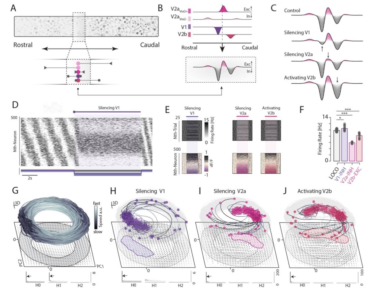
🧠 New #preprint by Komi et al. (2025): Neural #manifolds that orchestrate walking and stopping. Using #Neuropixels recordings from the lumbar spinal cord of freely walking rats, they show that #locomotion arises from rotational #PopulationDynamics within a low-dimensional limit-cycle #manifold. When walking stops, the dynamics collapse into a postural manifold of stable fixed points, each encoding a distinct pose.

🌍 https://doi.org/10.1101/2025.11.08.687367

#CompNeuro #NeuralDynamics #Attractor #Neuroscience

Neural manifolds that orchestrate walking and stopping

Fig. 1. Model of spinal motor network and the walk-to-stop transitions: Bifurcation from limit cycle to a
fixed point attractor. — Fig. 1. Model of spinal motor network and the walk-to-stop transitions: Bifurcation from limit cycle to a fixed point attractor.

Fabrizio Musacchio

@pixeltracker@sigmoid.social · 5 days ago

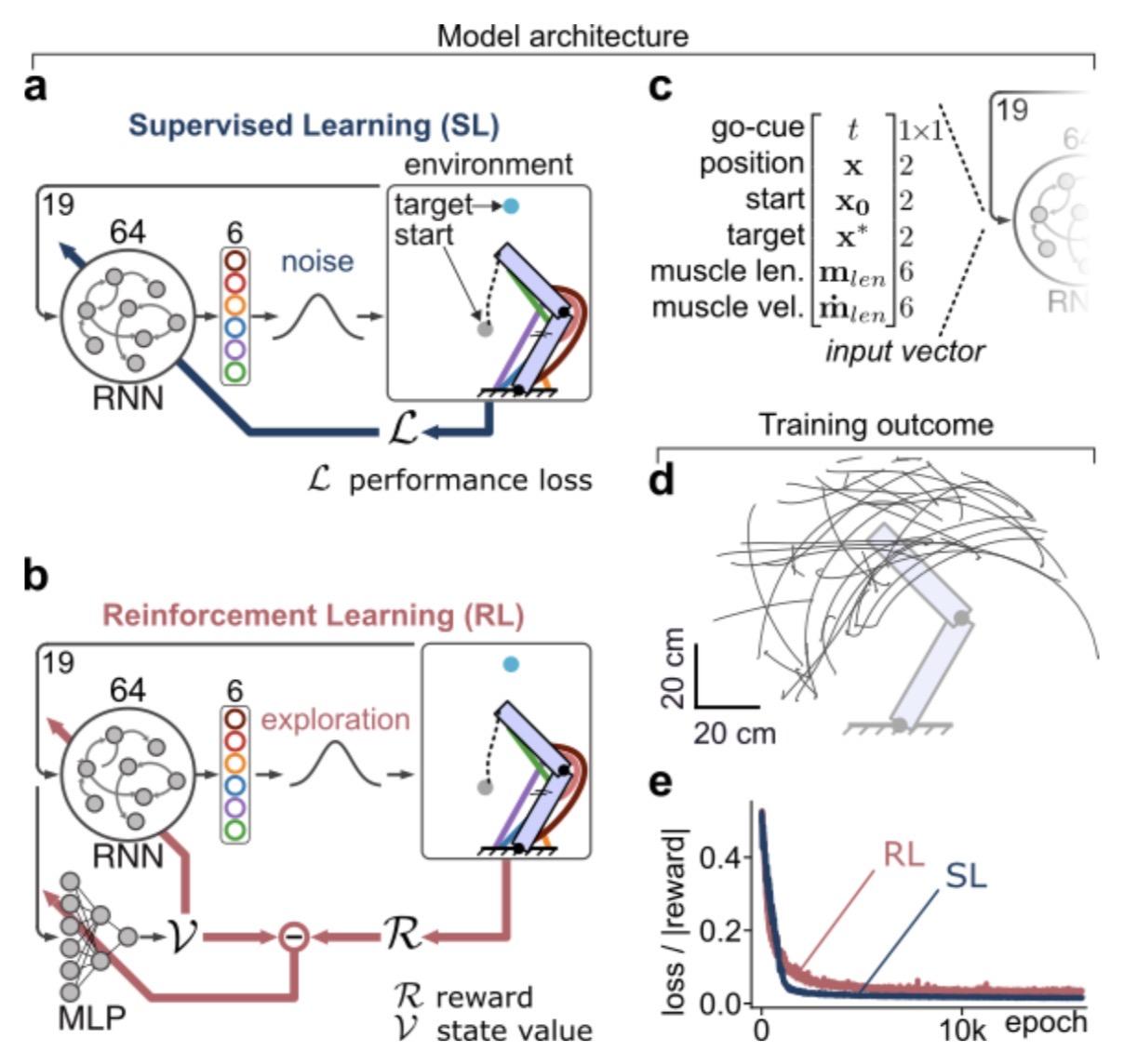
🧠 New preprint by Codol et al. (2025): Brain-like #NeuralDynamics for #behavioral control develop through #ReinforcementLearning. They show that only #RL, not #SupervisedLearning, yields neural activity geometries & dynamics matching monkey #MotorCortex recordings. RL-trained #RNNs operate at the edge of #chaos, reproduce adaptive reorganization under #visuomotor rotation, and require realistic limb #biomechanics to achieve brain-like control.

🌍 https://doi.org/10.1101/2024.10.04.616712

#CompNeuro #Neuroscience

Brain-like neural dynamics for behavioral control develop through reinforcement learning

Fig. 2: Neural networks trained with RL or SL achieved high performance in controlling the effector .

Fabrizio Musacchio

@pixeltracker@sigmoid.social · last week

🧠 New paper by Clark et al. (2025) shows that the #dimensionality of #PopulationActivity in #RNN can be explained by just two #connectivity parameters: effective #CouplingStrength and effective #rank. Uses networks with rapidly decaying singular value spectra and structured overlaps between left and right singular vectors. Could be useful for interpreting large scale population recordings and connectome data I guess:

🌍 https://doi.org/10.1103/2jt7-c8cq

#CompNeuro #NeuralDynamics #Connectome

Connectivity Structure and Dynamics of Nonlinear Recurrent Neural Networks

Fig. 2.
Schematic of the random-mode model. Upper: couplings
J
are generated as a sum of outer products,
ℓ
a
r
a
T
, with component strengths
D
a
. Lower: the two-point function
C
⋆
ϕ
(
τ
)
and four-point function
Ψ
⋆
ϕ
(
τ
)
are calculated in terms of the statistics of
D
a
. The two-point function depends only on the effective gain
g
eff
, while the four-point function depends on both
g
eff
and
PR
D
, the effective dimension of the connectivity determined by the
D
a
distribution. — Fig. 2. Schematic of the random-mode model. Upper: couplings J are generated as a sum of outer products, ℓ a r a T , with component strengths D a . Lower: the two-point function C ⋆ ϕ ( τ ) and four-point function Ψ ⋆ ϕ ( τ ) are calculated in terms of the statistics of D a . The two-point function depends only on the effective gain g eff , while the four-point function depends on both g eff and PR D , the effective dimension of the connectivity determined by the D a distribution.